Tutorial: Cohort Analysis with Imply

Imagine you are running an online gaming platform where players deposit funds into their accounts and then use these funds for games. In order to analyze player retention and lifetime value, you want to group players according to when they signed up (which calendar month, or week), and then for each group chart their spending behaviour over time, starting at the time when they signed up.
This is the use case for cohort analysis.
Cohort analysis is also used to analyze customer loyalty in ecommerce, and there are numerous other application cases in various industries. With Imply, it is easy to do even on large data sets.
Let’s look at an example!
In this tutorial, you will
- Generate a random data set that is suitable for cohort analysis
- Ingest this data set into Imply Polaris
- Create a suitable logical data model in Imply Pivot, on top of the Druid table
- Create a cohort based visualisation.
Simulating Data
Let’s create a simple data set. The following script creates a random set of players with signup dates in the last 2 years, and then generates events, trying to mimic typical player behaviour by creating fewer events for players that have been with the platform for a longer time.
Each event row describes a deposit made, and includes the event date, the player ID, the player’s signup date, and the amount of the deposit.
Run the Perl 5 script below and pipe the output into a file named cohort.csv:
#!/usr/bin/perl
# create data set for cohort analysis

use strict;
use warnings;

use Getopt::Std;
use DateTime;

my $start = DateTime->new(
    day   => 1,
    month => 1,
    year  => 2022,
);

my $stop = DateTime->new(
    day   => 1,
    month => 9,
    year  => 2022,
);

my $numPlayers = 100000;
my $playerMaxAge = 730;
my $minEventsPerDay = 300;
my $maxEventsPerDay = 1000;
my $maxDeposit = 50;

my @players;
my @playerSignup;

my $today = DateTime->today;

# initialize players and signup dates

for my $i (0 .. $numPlayers-1 ) {
    my $playerID = "p" . sprintf("%05d", $i);
    $players[$i] = $playerID;
    my $playerAgeNow = int(rand($playerMaxAge));
    my $signupDate = $today - DateTime::Duration->new(days => $playerAgeNow);
    $playerSignup[$i] = $signupDate;
}

print "curdate,playerid,signupdate,deposit\n";

for ( my $d = $start->clone; $d < $stop; $d->add(days => 1) ) {
    my $n = 0;
    my $numEventsMax = $minEventsPerDay + int(rand($maxEventsPerDay - $minEventsPerDay));
    while ($n < $numEventsMax) {
        my $ind = int(rand($numPlayers));
        my $playerID = $players[$ind];
        next if ( $playerSignup[$ind] > $d ); # player did not exist yet

        my $playerAge = $d->delta_days($playerSignup[$ind])->in_units('days');
        my $cooldown = exp(-3.0 * $playerAge / $playerMaxAge);
        next if ( rand(1.0) > $cooldown ); # simulate that players churn off slowly

        my $deposit = sprintf("%.2f", rand($maxDeposit));
        print "$d,$playerID,$playerSignup[$ind],$deposit\n";
        ++$n;
    }
}
Ingesting the Data
Here you can find instructions how to sign up for a free trial of Imply Polaris. After following the signup process, you will have a fresh Polaris environment.
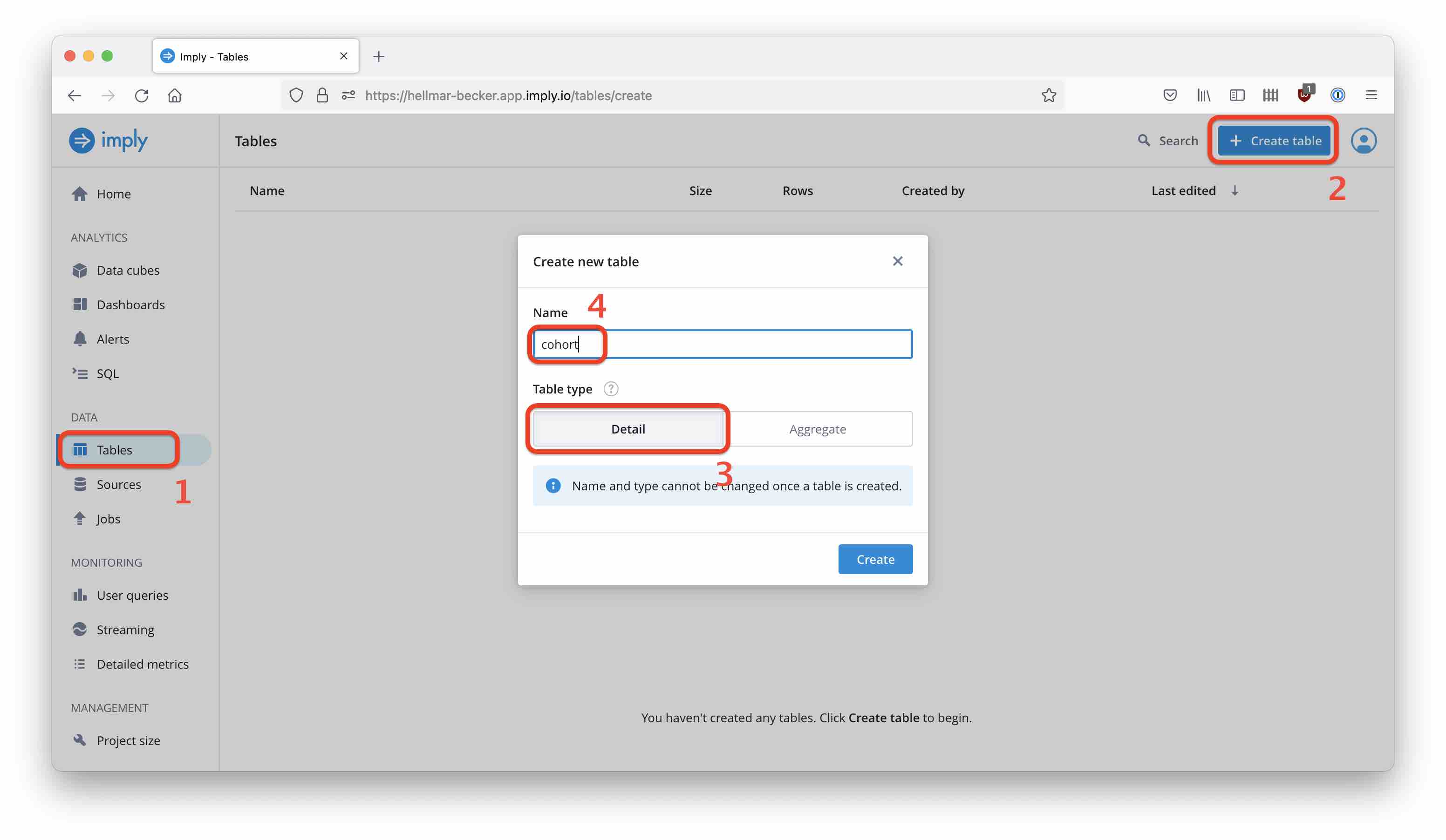
Let’s create a table. Select Tables from the left navigation bar and start the table creation wizard using the Create table button. Name the new table cohort and make sure Detail is selected.
(There are two kinds of tables in Polaris, Detail and Aggregate. Detail tables store the individual rows as they occur in the source data. Aggregate tables correspond to what we call rollup in Druid, where data is aggregated to a predefined time granularity, greatly reducing storage needs. One of the cool things in Druid and Polaris is that you can have that level of aggregation and still count unique things, like visitors. But for now, we need the detail data.)
Select Load data to define your new table’s schema based on the sample file. This will take you to the data sources dialog, where you select Files and Upload files from your computer. Select the cohort.csv file from the previous step, wait until the upload completes and proceed to the next step.
You will be presented with a sample from your data which should look similar to this:
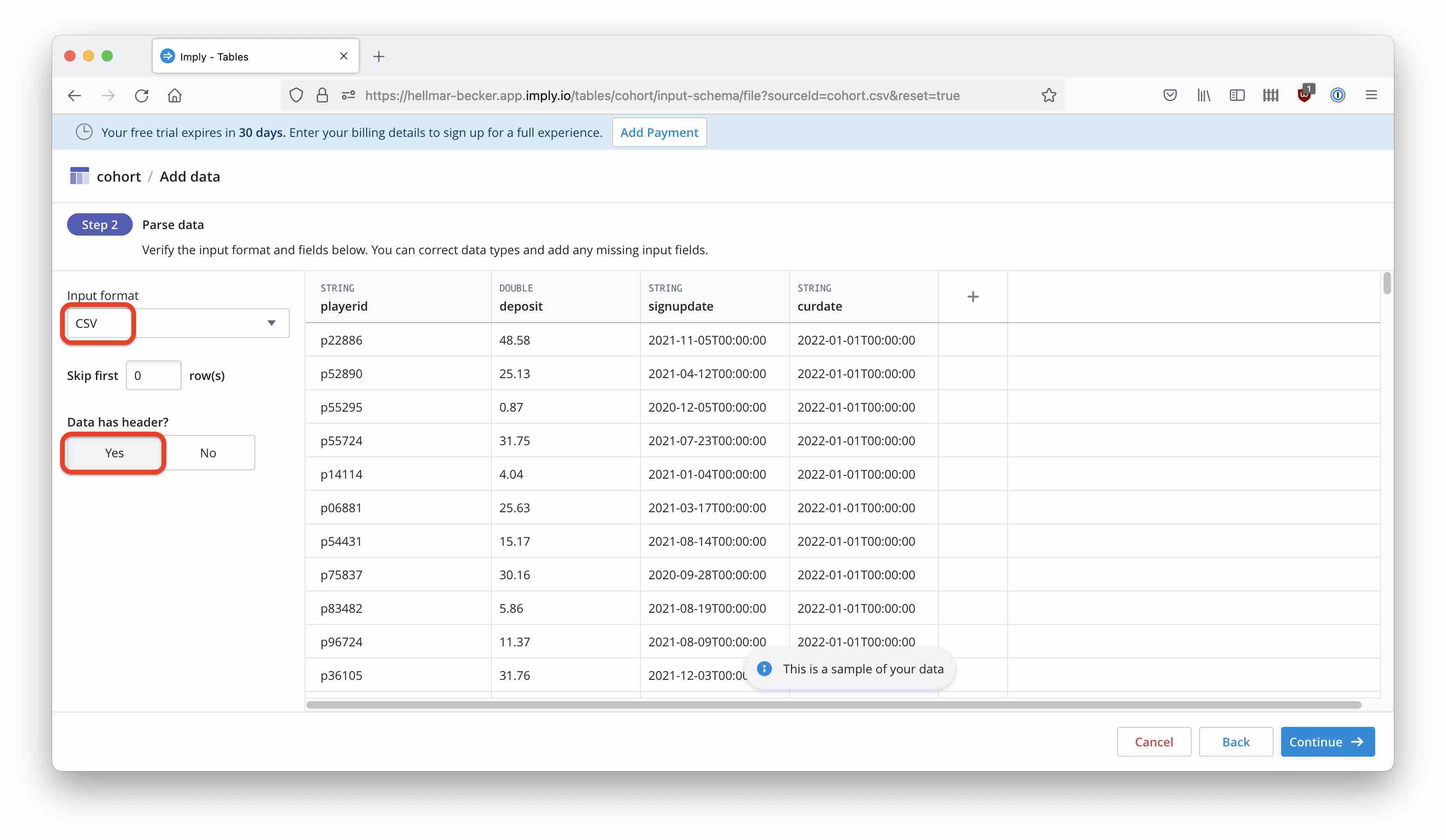
Verify that the input format is CSV and the Data has header switch is set to Yes. Continue to the next step:
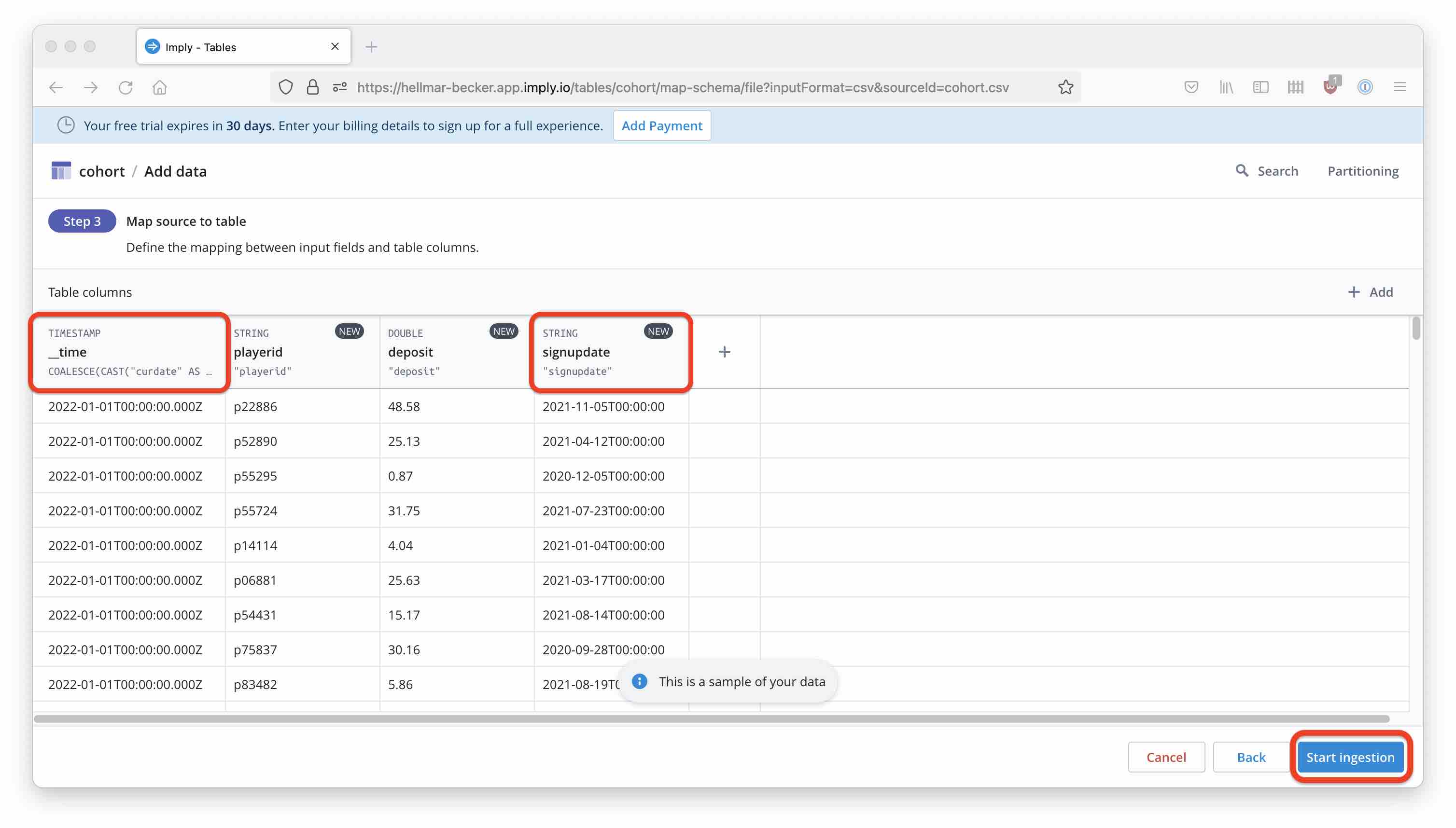
Make sure the primary timestamp (__time) is derived from the curdate column, and the signupdate field is modeled as a string. Then start the ingestion. After a short while, you can see how the table is populated with data.
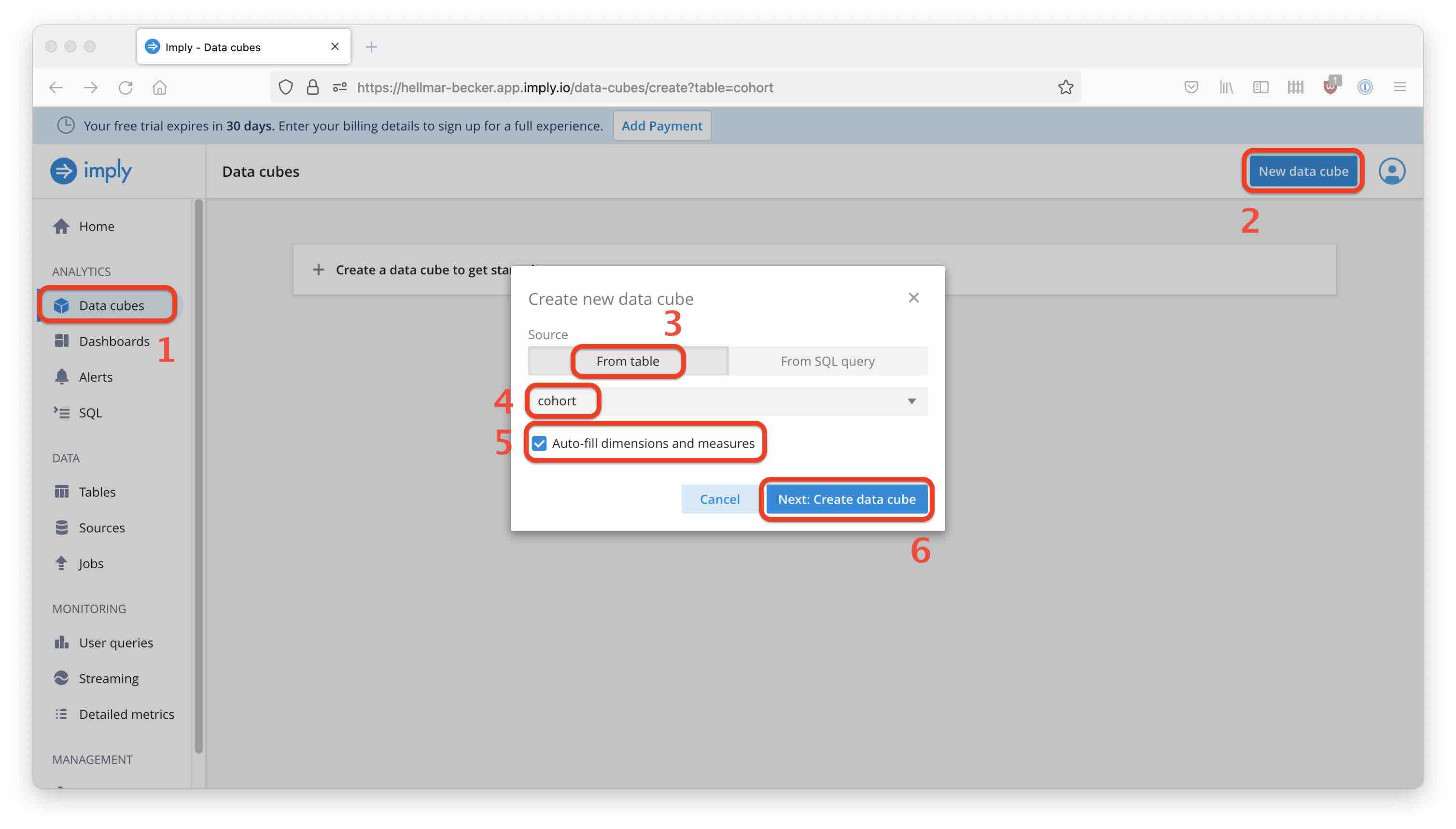
Creating the Logical Data Model
From the Data cubes navigation item, go to New data cube. Create a data cube from your new table and have it prepopulated by the wizard:
Measures
- A default
SUMmeasure over the deposits has been created automatically. This is fine for the tutorial; in a real life scenario you would have to consider rolled back deposits and other special cases as well. - The number of events is always present as a
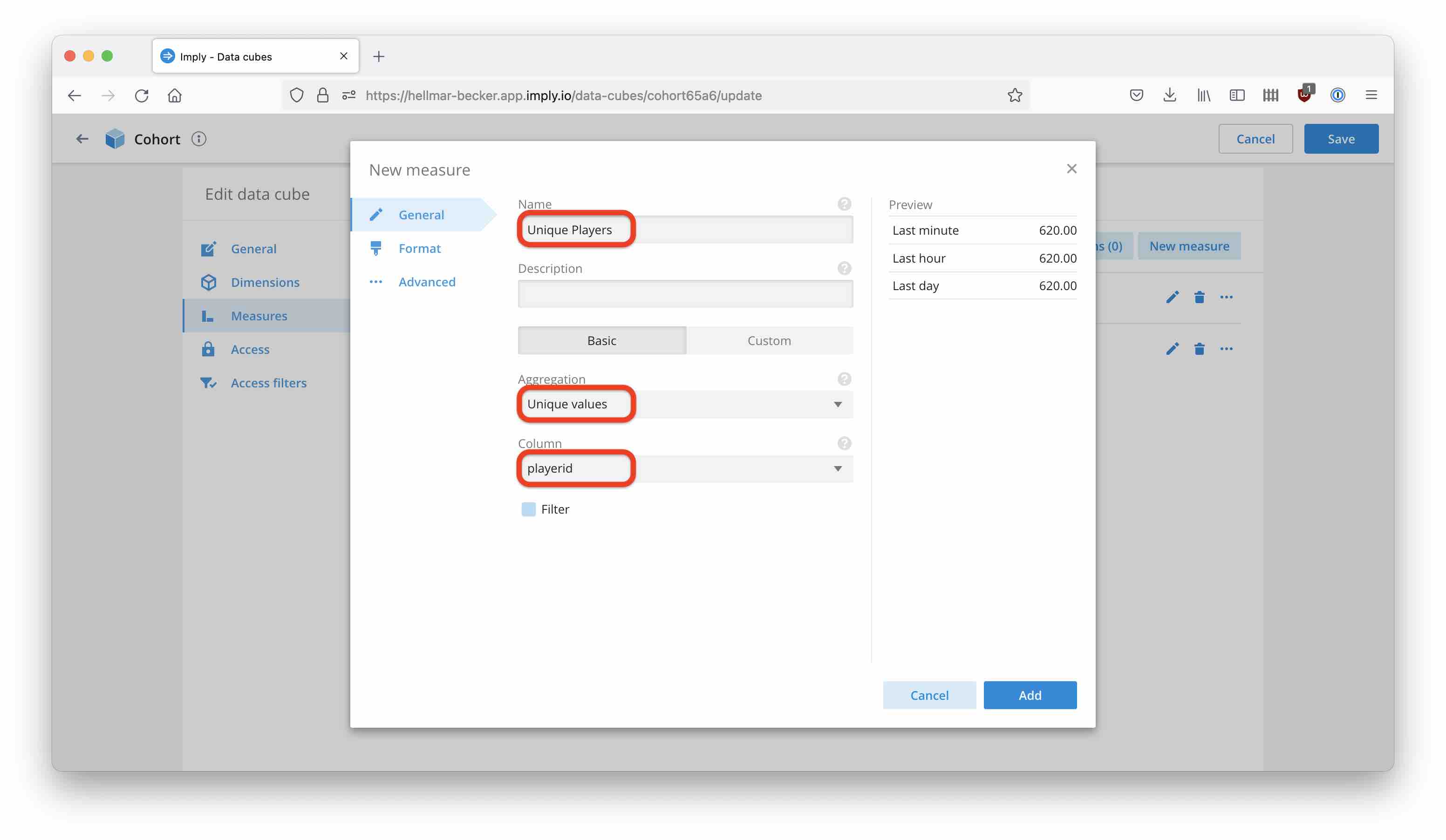
COUNTmeasure. - Add a measure to count unique players:
Dimensions
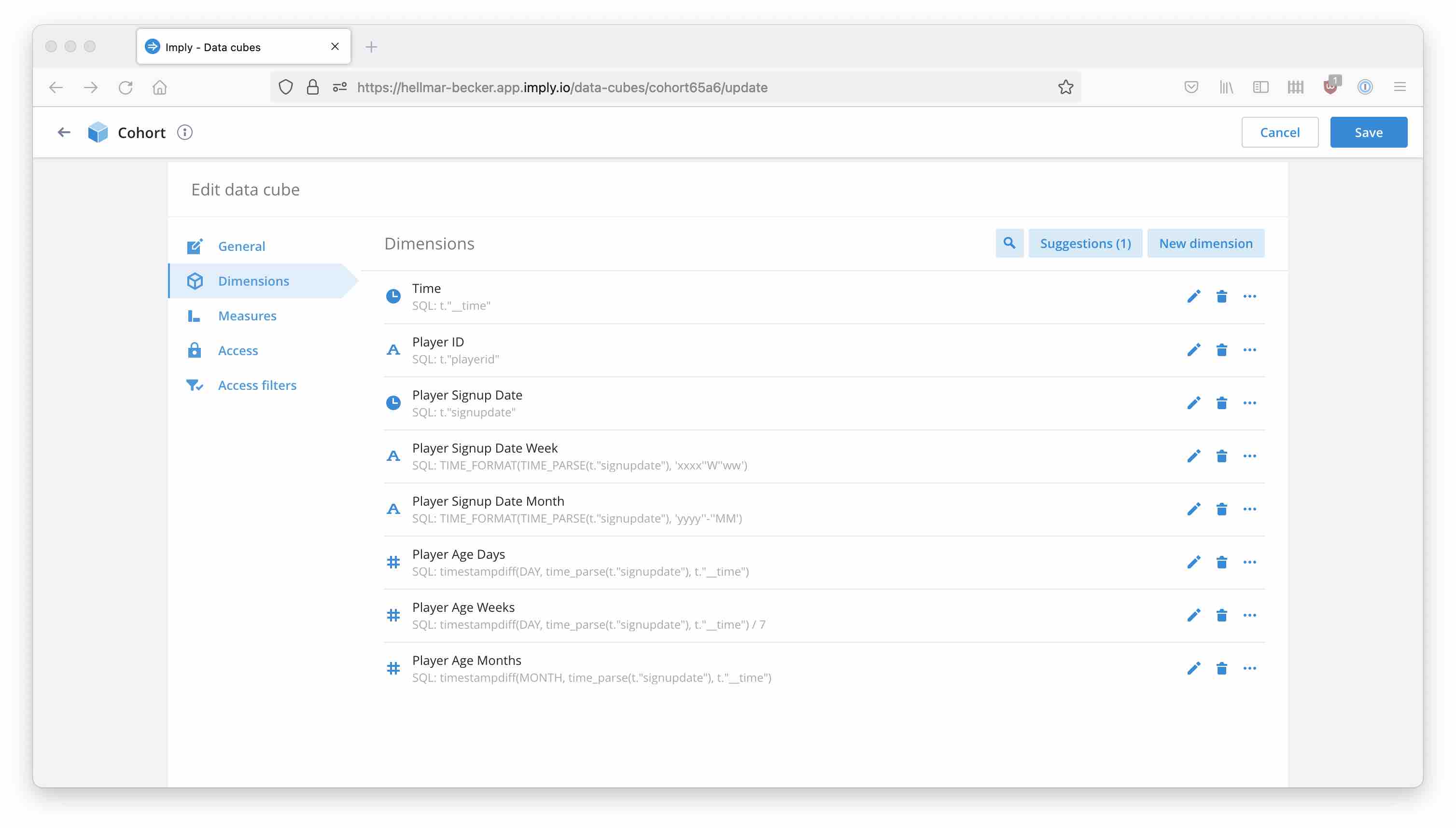
We are going to add some enhancements to the logical data model.
- Change the data type of the signup date column to
Timeso we can have a date selector on it. (Pivot will automatically parse and convert the datetime string.) I am also renaming the dimensions toPlayer IDandPlayer Signup Dateto make the reports look nicer. - In order to group the players into cohorts by their signup date, parse out the month and calendar week from the signup date. Note that in order to match with the calendar week, you need to use the week year (
'xxxx') date mask rather that'yyyy'. - Add
Player Ageas the time between event time and signup time as a set of calculated dimensions in days, weeks, and months. These are numbers but make sure to disable default bucketing.
Add the following dimensions:
| Dimension Name | Data Type | Formula | Possible bucketing |
|---|---|---|---|
| Player Signup Date Week | String | TIME_FORMAT(TIME_PARSE(t."signupdate"), 'xxxx''W''ww') |
- |
| Player Signup Date Month | String | TIME_FORMAT(TIME_PARSE(t."signupdate"), 'yyyy''-''MM') |
- |
| Player Age Days | Number | TIMESTAMPDIFF(DAY, TIME_PARSE(t."signupdate"), t."__time") |
Never bucket |
| Player Age Weeks | Number | TIMESTAMPDIFF(DAY, TIME_PARSE(t."signupdate"), t."__time") / 7 |
Never bucket |
| Player Age Months | Number | TIMESTAMPDIFF(MONTH, TIME_PARSE(t."signupdate"), t."__time") |
Never bucket |
(If you leave bucketing on, you will have to switch it off explicitly every time you build a chart, and we want the individual values in any case. You could achieve the same using a String dimension but that would mess up the sort order.)
After that, your data model should look like this:
Creating the Cohort Chart
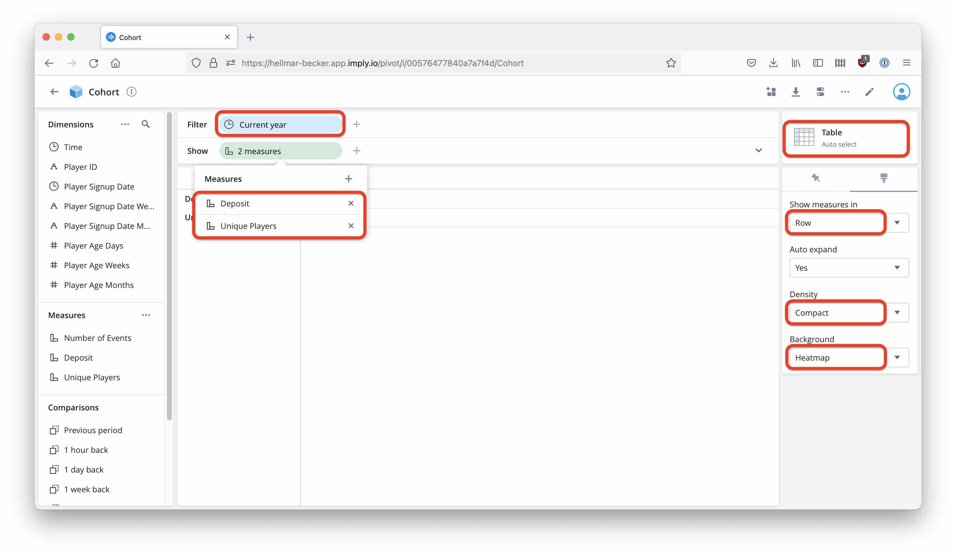
In the Cube view, select a Table visualisation. Set the time filter to Current year, select Deposit and Unique players as measures, and set the formatting options as shown.
Expand the Show bar and drag Player Signup Date Month into the Rows. Make sure the sort order is ascending by Player Signup Date Month.
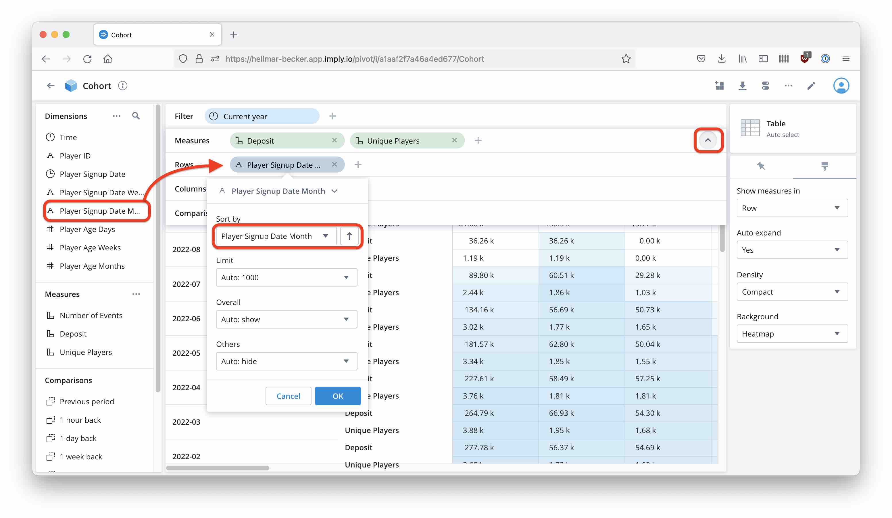
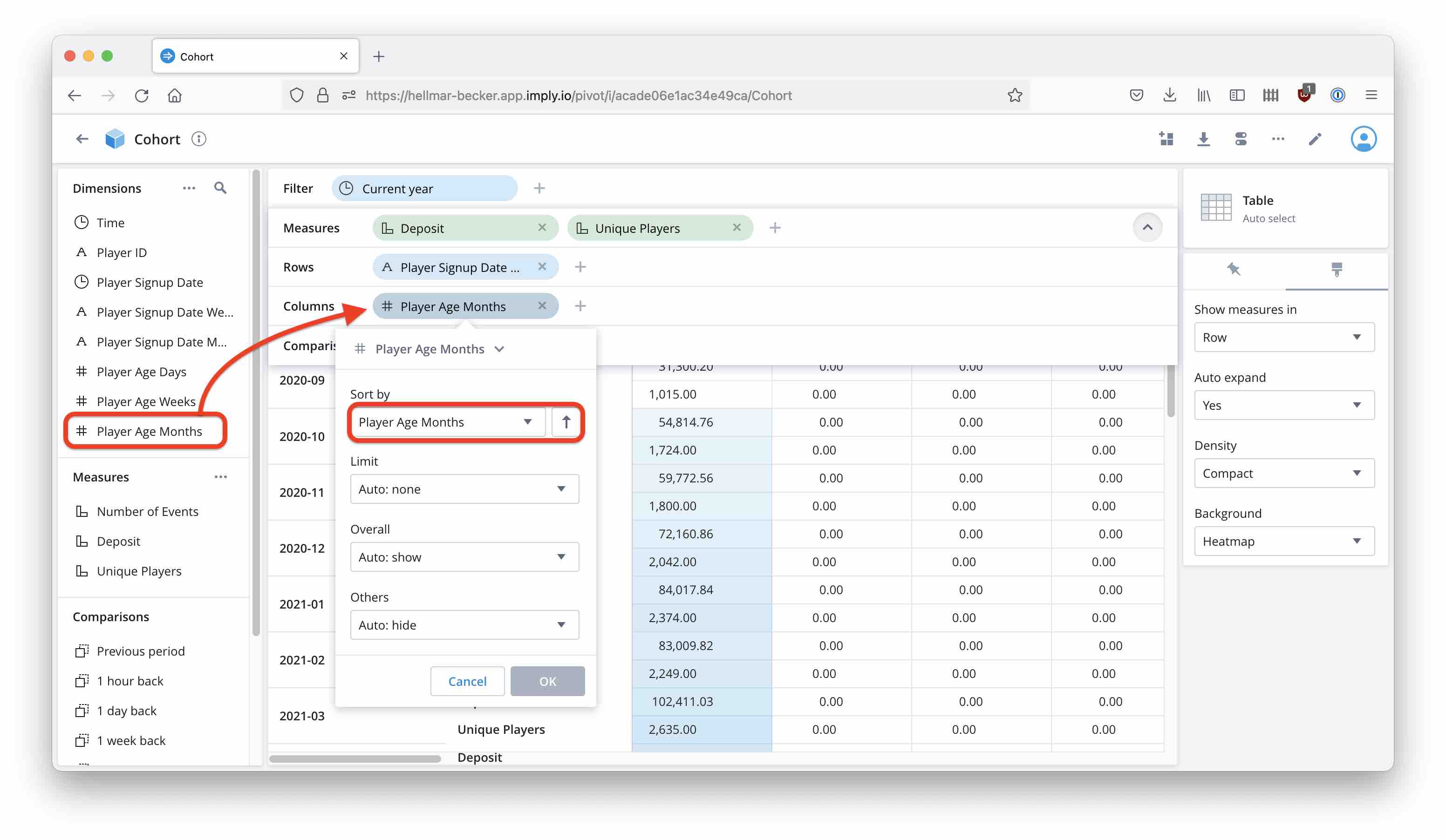
Likewise, add Player Age Months to the Columns section.
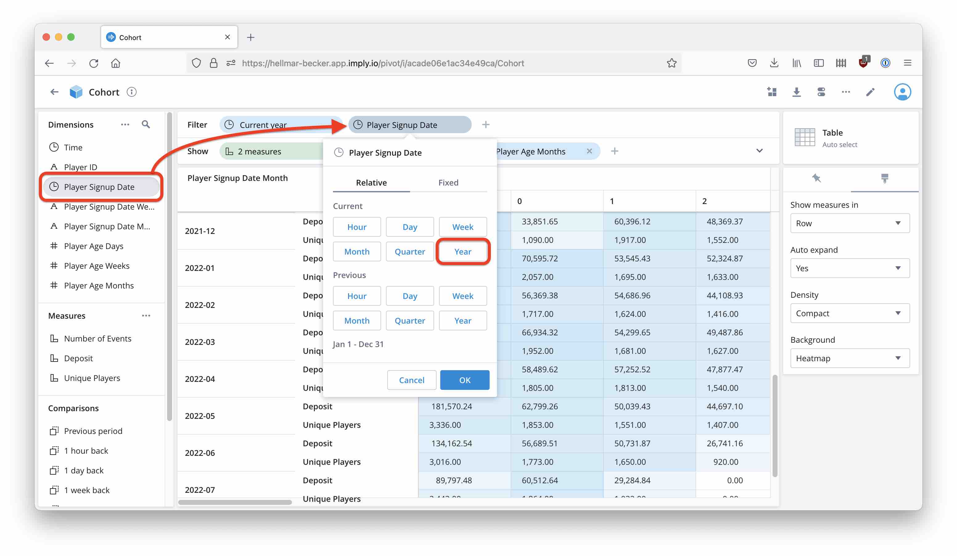
Set a filter on signup date, using the time dimension for signup date:
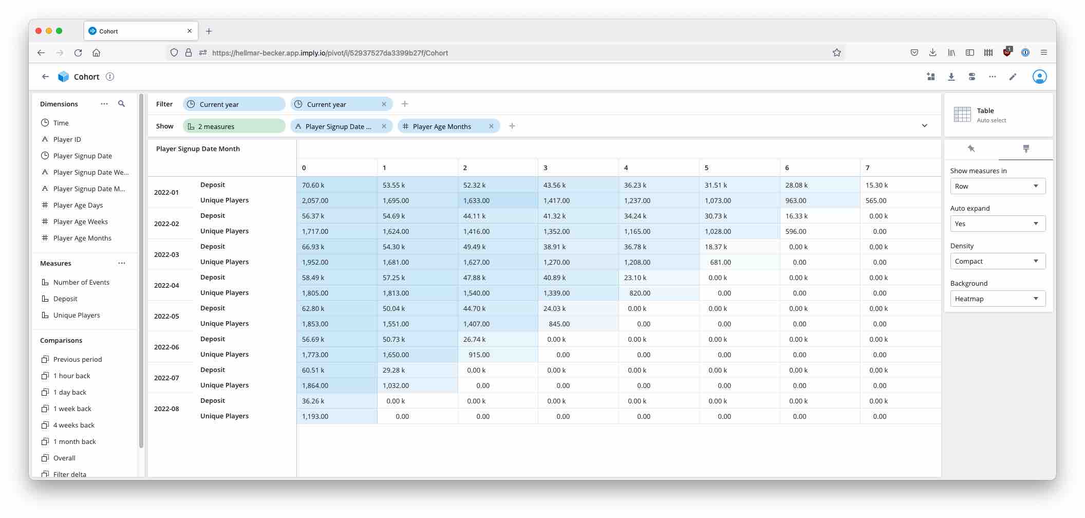
Here’s the final result, as it looks on the big screen and with totals hidden:
The same analysis can be done on a calendar week basis, showing the relative player age in weeks as well. This is left as an exercise for the reader.
Learnings
- Imply Polaris lets you build analytics powered by Druid with just a few easy steps.
- Imply Pivot allows secondary timestamp dimensions that are based on ISO formated timestamp strings.
- Time differences can be analyzed using computed dimensions.
- With these elements, it is easy to show a graphical cohort analysis.
"Roulettetisch im Casino" by marcoverch is licensed under CC BY 2.0 ![]()
![]() .
.