Partitioning in Druid - Part 1: Dynamic and Hash Partitioning
In addition to segmenting data by time, Druid allows to introduce secondary partitioning within each time chunk. There are various strategies:
- dynamic partitioning
- hash partitioning
- single dim partitioning
- new in Druid 0.22: range (or multi dim) partitioning.
I am going to take a look at each of these in the next few posts.
Let’s use the Wikipedia sample data to do some experiments. You can use the Druid quickstart for this tutorial.
Dynamic Partitioning
Generally speaking, dynamic partitioning does not do a lot to the data with regards to organizing or reordering them. You will get one or more partitions per input data blob for batch ingestion, and one or more partitions per Kafka partition for realtime Kafka ingestion. Often times, the resulting segment files are smaller than desired. The upside of this strategy is that ingestion with dynamic partitioning is faster than any other strategy, and it doesn’t need to buffer or shuffle data. The downside is that it doesn’t do anything to optimize query performance.
For the first experiment, follow the quickstart tutorial step by step, with one exception: Set the maximum number of rows per segment to 14,000, because we want to have more than one partition:
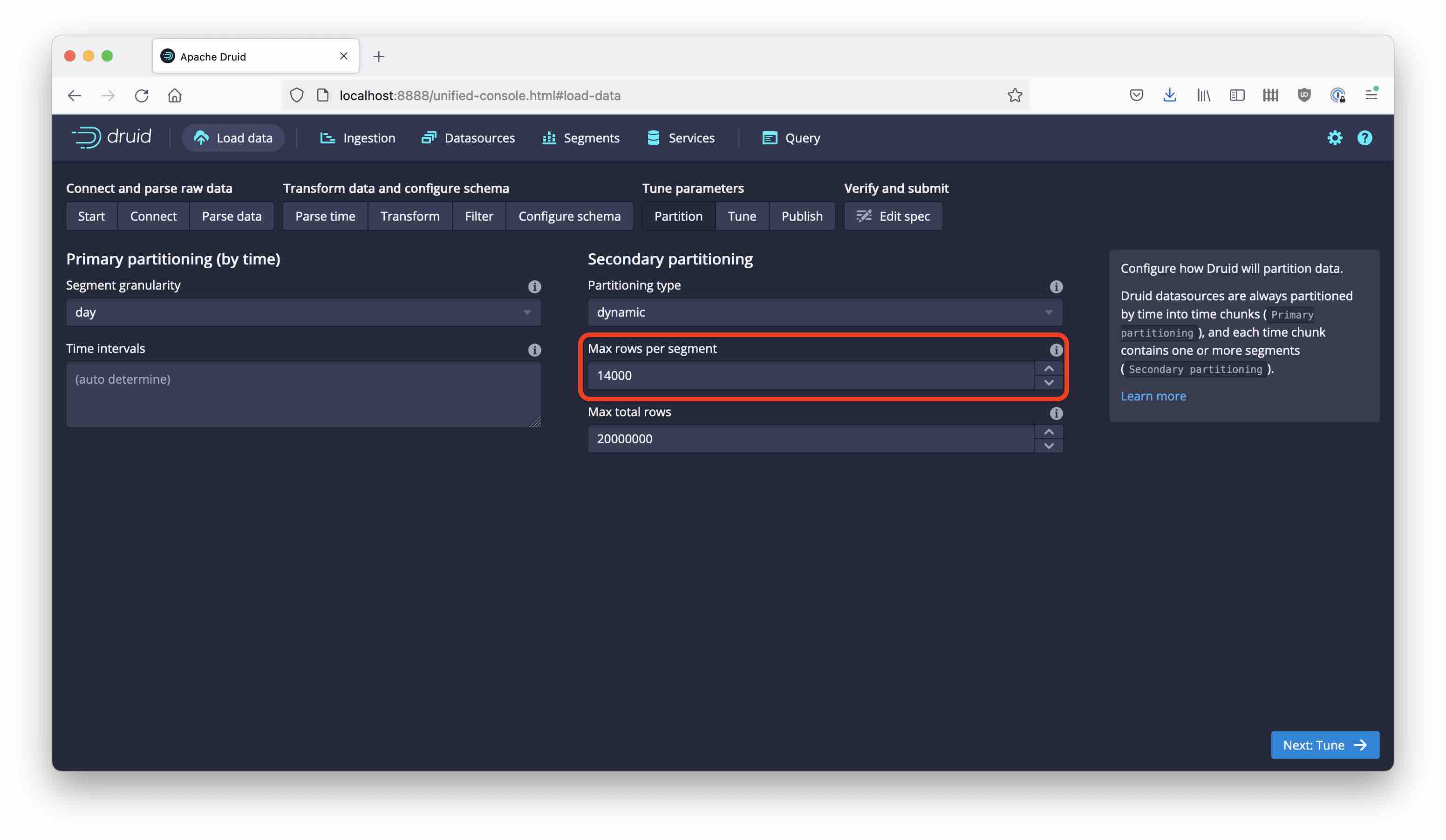
Also, name the datasource wikipedia-dynamic-1 (we will create more versions of this.) Run the ingestion, it will finish within a few seconds. Now let’s look what we have:
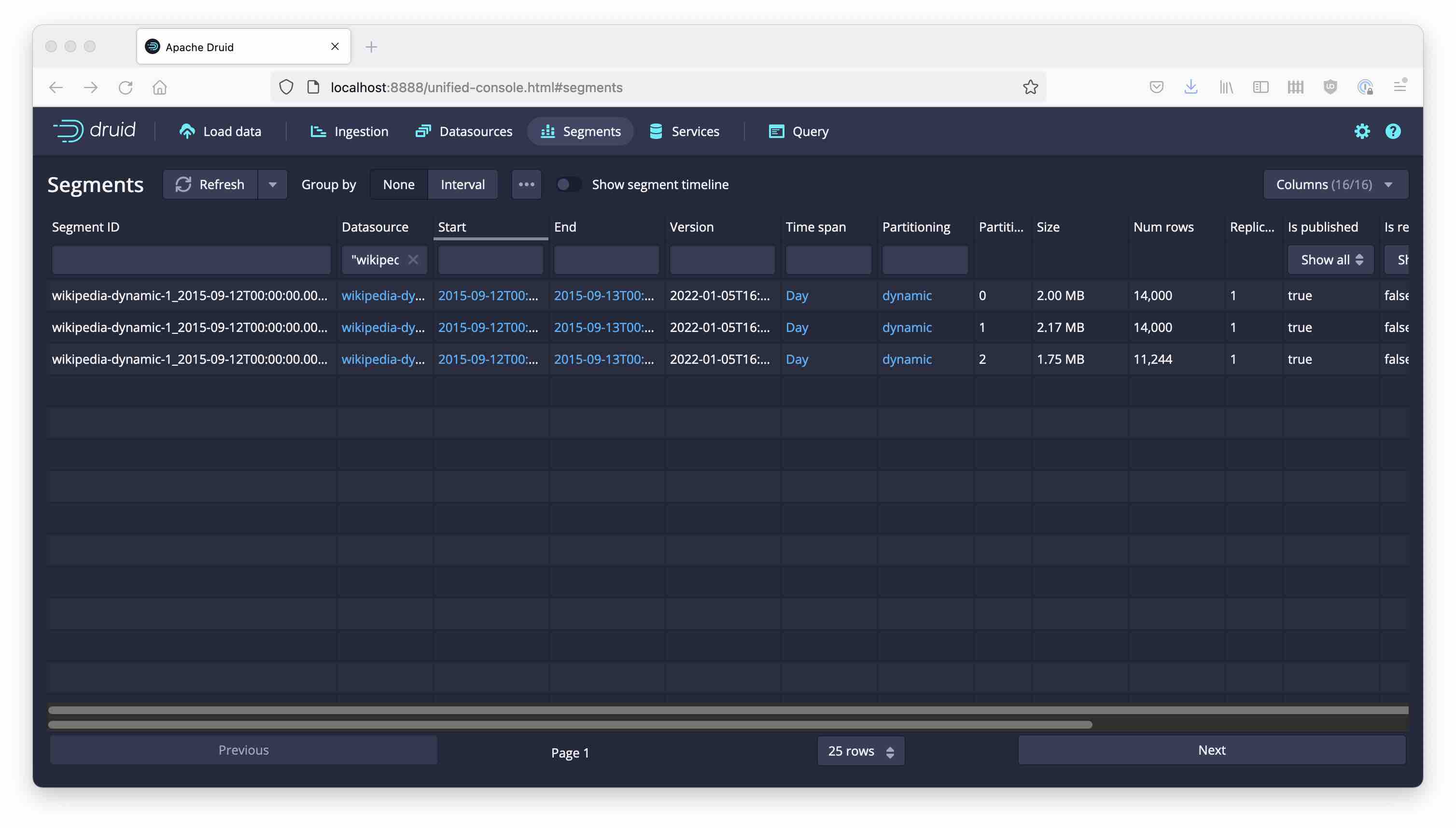
Because the sample has roughly 40,000 rows of data, Druid has created three partitions. Let’s take a closer look at the partitions.
In the quickstart setup, the segments live in var/druid/segments/, and here’s the structure Druid has created for the new datasource:
wikipedia-dynamic-1
└── 2015-09-12T00:00:00.000Z_2015-09-13T00:00:00.000Z
    └── 2022-01-05T16:03:35.016Z
        ├── 0
        │   └── index.zip
        ├── 1
        │   └── index.zip
        └── 2
            └── index.zip
So, we have datasource-name / time chunk / version timestamp / partition number. Each leaf file is a zip archive with the segment data, the format is described here.
Druid comes with a dump-segment tool, which has a number of interesting options. But in order to use it, we need to unzip the index.zip files first. Let’s dump the data and look at the distribution of one dimension: I am going to pick the channel dimension, because it is well populated and has a limited number of values that occur frequently.
#!/bin/bash

# path settings for default quickstart install

DRUID_HOME="${HOME}/apache-druid-0.22.1"
DRUID_DATADIR="${DRUID_HOME}/var/druid/segments"
DRUID_DATASOURCE="wikipedia-dynamic-1"
DUMP_TMPDIR="${HOME}/tmpwork"

TOPN=5

FILES=$(cd ${DRUID_DATADIR} && find ${DRUID_DATASOURCE} -type f)

for f in $FILES; do
  FDIR=$(dirname $f)
  FBASE=$(basename $f)
  PARTN=$(cut -d "/" -f 4 <<<$f)
  ODIR=${DUMP_TMPDIR}/$FDIR
  mkdir -p $ODIR
  unzip -q -o ${DRUID_DATADIR}/$f -d $ODIR

  java -classpath "${DRUID_HOME}/lib/*" -Ddruid.extensions.loadList="[]" org.apache.druid.cli.Main \
    tools dump-segment \
    --directory $ODIR \
    --out $ODIR/output.txt

  # Top Countries Report
  echo Partition $PARTN:
  jq -r ".channel" $ODIR/output.txt | sort | uniq -c | sort -nr | head -$TOPN

done
And here is the output that I get:
Partition 0:
4476 #vi.wikipedia
4061 #en.wikipedia
 650 #zh.wikipedia
 638 #de.wikipedia
 514 #it.wikipedia
Partition 1:
3854 #en.wikipedia
3152 #vi.wikipedia
1080 #de.wikipedia
 921 #fr.wikipedia
 597 #it.wikipedia
Partition 2:
3634 #en.wikipedia
2119 #vi.wikipedia
 872 #uz.wikipedia
 805 #de.wikipedia
 730 #fr.wikipedia
The most frequent values are all scattered over all partitions! This way, even if a query filters on a single channel value, it will have to read all segments. And for a group by query, all the groups will have to be assembled in the query node. This partitioning strategy does not make queries any faster.
Hash Partitioning
Now, let’s try something different.
Hash partitioning computes a hash key based on a set of one or more dimension values, and assigns the partition based on that key. What are the consequences?
Set the partitioning to hashed, and enter channel for the dimensions. Also set the target rows to 14,000, so we get three partitions again.
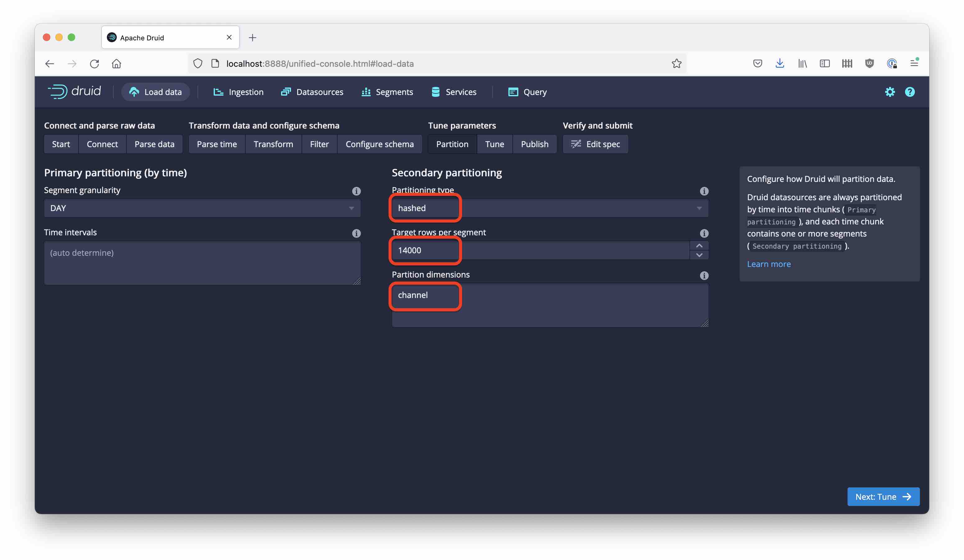
For good measure, name this datasource wikipedia-hashed. Running the same analysis as above gives this result:
Partition 0:
11549 #en.wikipedia
2099 #fr.wikipedia
1126 #zh.wikipedia
 472 #pt.wikipedia
 445 #nl.wikipedia
Partition 1:
2523 #de.wikipedia
1386 #ru.wikipedia
1256 #es.wikipedia
 533 #ko.wikipedia
 478 #ca.wikipedia
Partition 2:
9747 #vi.wikipedia
1383 #it.wikipedia
 983 #uz.wikipedia
 749 #ja.wikipedia
 565 #pl.wikipedia
We got segments of roughly the same size, and each value of channel ends up in only one segment. However, as a rule, similar values of the partition key do not end up in the same segment. Thus, range queries will not benefit. Queries with a single value filter can be faster, though. Also, TopN queries will give more accurate results than with dynamic partitioning.
Conclusion
So, why would you even use dynamic partitioning? There are two reasons, or maybe three:
- If you are ingesting realtime data, you need to use dynamic partitioning.
- Also, you can always add (append) data to an existing time chunk with dynamic partitioning.
- The third reason: you do not need to reshuffle data between partitions, so ingestion is faster and less resource intensive than with other partitioning schemes.
Hash partitioning helps ensure a proper distribution of the data, but has limited query performance benefits.
For query optimization, we have to look at the remaining partitioning schemes. Stay tuned!
“Remedy Tea Test tubes” by storyvillegirl is licensed under CC BY-SA 2.0, cropped and edited by me